Rearrangement of climate zones and the emergence of novel climate profiles during this century will have substantial ramifications for biodiversity. While all species currently on earth persisted through previous periods of climate change by migration or adaptation, landscapes today are frequently highly fragmented, and contemporary climate change is taking place at a pace that likely exceeds the adaptive capacity of biodiversity. These factors will make it increasingly difficult for some populations and species to continue to persist in their current ranges. Indeed, there is already strong evidence from Australia3 and elsewhere documenting shifts in species distributions due to anthropogenic climate change4. Of key concern, from a species management perspective, is understanding how suitable habitat for a given species may be altered in the future.
As the climate changes, areas currently suitable for a species may become unsuitable, while locations that are currently unsuitable may now have conditions that species can tolerate. Hence, habitat may be lost or gained. Understanding which populations are more (or less) vulnerable to changes in climate is of key concern to conservation and land managers.
From a climate change perspective, refugia are areas where species can retreat to and persist in under changing environmental conditions5. In other words, refugia are areas that maintain favourable climatic conditions absent in the surrounding landscape5,6, thereby safeguarding the persistence of biodiversity. This means that refugia are critical components in climate change management and adaptation planning7, and their identification and protection is increasingly a priority for conservation managers.
Two key types of refugia, termed internal or external, are determined by their spatial relationship with species' known distributions. In this project, internal refugia can be identified as occurring in areas where a) there are currently populations of the target species and b) those areas remain suitable in future conditions. External refugia are regions in which populations are currently absent but are projected to be suitable in the future. However, although a region may contain conditions suitable for the species, this does not guarantee that populations will be able to disperse or persist on those areas.

Figure 1. Schematic diagram illustrating the concept of internal and external refugia. On the left, the current range of a hypothetical species is demonstrated. As climate changes, part of this range will likely become unsuitable, leading to extinction of populations (hatched area on the right). However, some parts of the range may continue to retain suitable climate and these areas are referred to as internal refugia. Areas that were previously unsuitable may also become suitable in the future, and these areas can be classified as external refugia (i.e. they are external to the species' current range).
Habitat suitability models (HSM), also called species distribution models (SDM), are statistical tools that can be used to generate spatial predictions of habitat suitability for species8. A HSM achieves this by identifying the relationship between where a species currently occurs and climate or environmental characteristics of those areas. HSMs are frequently used to examine the potential for changes to the spatial distribution of climatically suitable habitat under scenarios of future climate. This approach is based on the assumption that the locations of populations reflects the environmental preferences of a species8. As a result, HSMs can be used to a) identify currently suitable habitat for a target species; b) locate suitable habitat beyond the species' current range; and c) identify which geographic regions may be more, or less, suitable for the species in the future.

Figure 2. Schematic representation of how a correlative species distribution model (SDM) works. SDMs assess the relationship between where a species occurs and environmental variables at these locations (such as climate and soil). Models are created describing these relationships, and are then used to identify areas across the landscape that have conditions suitable for the species. The output of SDMs should NOT be interpreted as the actual distribution of the species. Rather, the output represents a hypothesis of what areas are suitable for the species given the environmental variables used in the model. In reality, other factors will influence a species' distribution, such as food, competition, disease, dispersal ability and barriers to dispersal.
Maps of habitat suitability should not be interpreted as actual distributions, as they consider only a limited number of variables that influence the likelihood of populations establishing and persisting in a region. It is likely that some areas identified as suitable by the HSM will not contain populations for myriad reasons including: vegetation type is unsuitable or habitat is unavailable; dispersal limitation or barriers; other biotic requirements or resources are not met. Users should utilise the maps in conjunction with other spatial data and expert knowledge.
While the maps provide a broad understanding of how climate change may alter habitat suitability, users should be aware that other factors influencing vulnerability to climate change are not including in the modelling process, including genetic adaptation, phenotypic plasticity, presence of micro-refugia, alterations to biotic interactions or future land-use changes.
We used data derived from climate simulations performed as part of the NSW and ACT Regional Climate Modelling (NARCliM) project9. The models project futures that we refer to as "Warmer/wetter", "Hotter/little change" in precipitation, "Hotter/wetter", and "Warmer/drier", given the future state with respect to mean annual temperature and annual precipitation of the baseline period (1990-2009). It is important to recognise that, at present, these futures are equally plausible. See the Methods for more information on these scenarios.
Table 1. Climate futures used in this study. Global Climate Models (GCM) assumed the SRES A2 emissions scenario10.
| Climate Future | GCM | Represents a future that is: |
|---|---|---|
| Warmer/Wetter | MIROC3.2(medres) | Warmer and wetter than present, particularly in NE NSW, although alpine regions are projected to become drier. |
| Hotter/Little change | ECHAM5/MPI-OM | Has the greatest increase in temperature, of the four scenarios. Precipitation trend varies across the state (slightly wetter in the NE and coastal regions, slightly drier elsewhere). |
| Hotter/Wetter | CCCMA CGCM3.1(T47) |
Warmer than MIROC, and wetter across most of the state, although areas in NW and SE of the state may be slightly drier. |
| Warmer/Drier | CSIRO-Mk3.0 | Warmer than present, and the driest of the four models. |
For each species, the following maps can be viewed on the website:
Table 2. Description of maps available on the website ClimateRefugiaNSW.
| Map | Range of Values | Description | Example |
|---|---|---|---|
| Current suitability (Continuous) | 0 to 1, where 0 = unsuitable and 1 = highly suitable | Distribution of suitable habitat in the baseline period (1991-2010) | 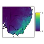 |
| Current suitability (Binary) | 0 or 1, where 0 = unsuitable and 1 = suitable | Distribution of suitable habitat in the baseline period (1991 - 2010) | 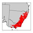 |
| Future suitability (Continuous) | 0 to 1, where 0 = unsuitable and 1 = highly suitable | Distribution of suitable habitat for each decade from 2010 to 2070. Four sets of maps are available, one for each of the future climate scenarios | 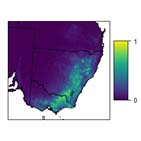 |
| Future suitability (Binary) | 0 or 1, where 0 = unsuitable and 1 = suitable | Distribution of suitable habitat for each decade from 2010 to 2070. Four sets of maps are available, one for each of the future climate scenarios | 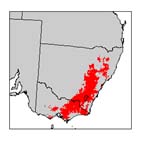 |
| Consensus | 0 to 4, where: 0 = unsuitable in all climate scenarios 1 = suitable in one climate scenario 2 = suitable in two climate scenarios ... and so on |
Agreement in binary suitability across the four climate scenarios. Maps are available for each decade from 2010 to 2070. This can be used to identify populations or regions that are projected to be vulnerable under all or none of the climate scenarios. | 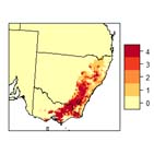 |
References
1. Phillips, S. J., Anderson, R. P. & Schapire, R. E. Maximum entropy modeling of species geographic distributions. Ecological Modelling 190, 231-259 (2006).
2. Phillips, S. J. & Dudík, M. Modeling of species distributions with Maxent: new extensions and a comprehensive evaluation. Ecography 31, 161-175 (2008).
3. Cabrelli, A., Beaumont, L. & Hughes, L. in Austral Ark (eds. Stow, A., Holwell, G. & Maclean, N.) (Cambridge University Press, 2015).
4. Pecl, G. T. et al. Biodiversity redistribution under climate change: Impacts on ecosystems and human well-being. Science 355, (2017).
5. Keppel, G. et al. Refugia: identifying and understanding safe havens for biodiversity under climate change. Global Ecology and Biogeography 21, 393-404 (2012).
6. Dobrowski, S. Z. A climatic basis for microrefugia: the influence of terrain on climate. Global Change Biology 17, 1022-1035 (2011).
7. Keppel, G. & Wardell-Johnson, G. W. Refugia: keys to climate change management. Global Change Biology 18, 2389-2391 (2012).
8. Franklin, J. Mapping species distributions: spatial inference and prediction. (Cambridge University Press, 2010).
9. Evans, J. P. et al. Design of a regional climate modelling projection ensemble experiment--NARCliM. Geoscientific Model Development 7, 621-629 (2014).
10. Nakicenovic, N. et al. Special report on emissions scenarios (SRES), a special report of Working Group III of the Intergovernmental Panel on Climate Change. (Cambridge University Press, 2000).
11. Rossel, R. A. V. & Chen, C. Digitally mapping the information content of visible-near infrared spectra of surficial Australian soils. Remote Sens. Environ. 115, 1443-1455 (2011).
12. Wilford, J. A weathering intensity index for the Australian continent using airborne gamma-ray spectrometry and digital terrain analysis. Geoderma 183-184, 124-142 (2012/8).
13. CSIRO. Topographic Wetness Index (3" resolution) derived from 1 second DEM-H version 1.0. (2012).
14. CSIRO. Topographic position index (3" resolution) derived from 1 second DEM-S version 0.1. (2012).
15. Elith, J. & Leathwick, J. R. Species distribution models: ecological explanation and prediction across space and time. Annual Review of Ecology, Evolution and Systematics 40, 677-697 (2009).
16. Elith*, J. et al. Novel methods improve prediction of species' distributions from occurrence data. Ecography 29, 129-151 (2006).
17. Elith, J. & Leathwick, J. Predicting species distributions from museum and herbarium records using multiresponse models fitted with multivariate adaptive regression splines. Diversity and Distributions 13, 265-275 (2007).
18. Swets, J. A. Measuring the accuracy of diagnostic systems. Science 240, 1285-1293 (1988).